Baeldung - CS

Learn all about Computer Science

What Are Gradient, Divergence, and Curl in Vector Calculus?
2025-07-15 22:24 UTC by Charles Udekwe

1. Introduction

In this tutorial, we’ll explore the concepts of gradient, divergence, and curl, learn the underlying math, and learn about their real-world applications.

2. Scalars, Vectors, Fields, and the Cartesian Coordinate System

In physics and math, quantities fall into scalars and vectors.

A scalar has only its magnitude (like time, mass, or temperature) while a vector includes both magnitude and direction, e.g., velocity or force.

Extending these to space, a field assigns values to every point in a region. Scalar fields provide a single value per point (e.g., room temperature), whereas vector fields assign direction and magnitude: imagine electromagnetic waves moving through the air.

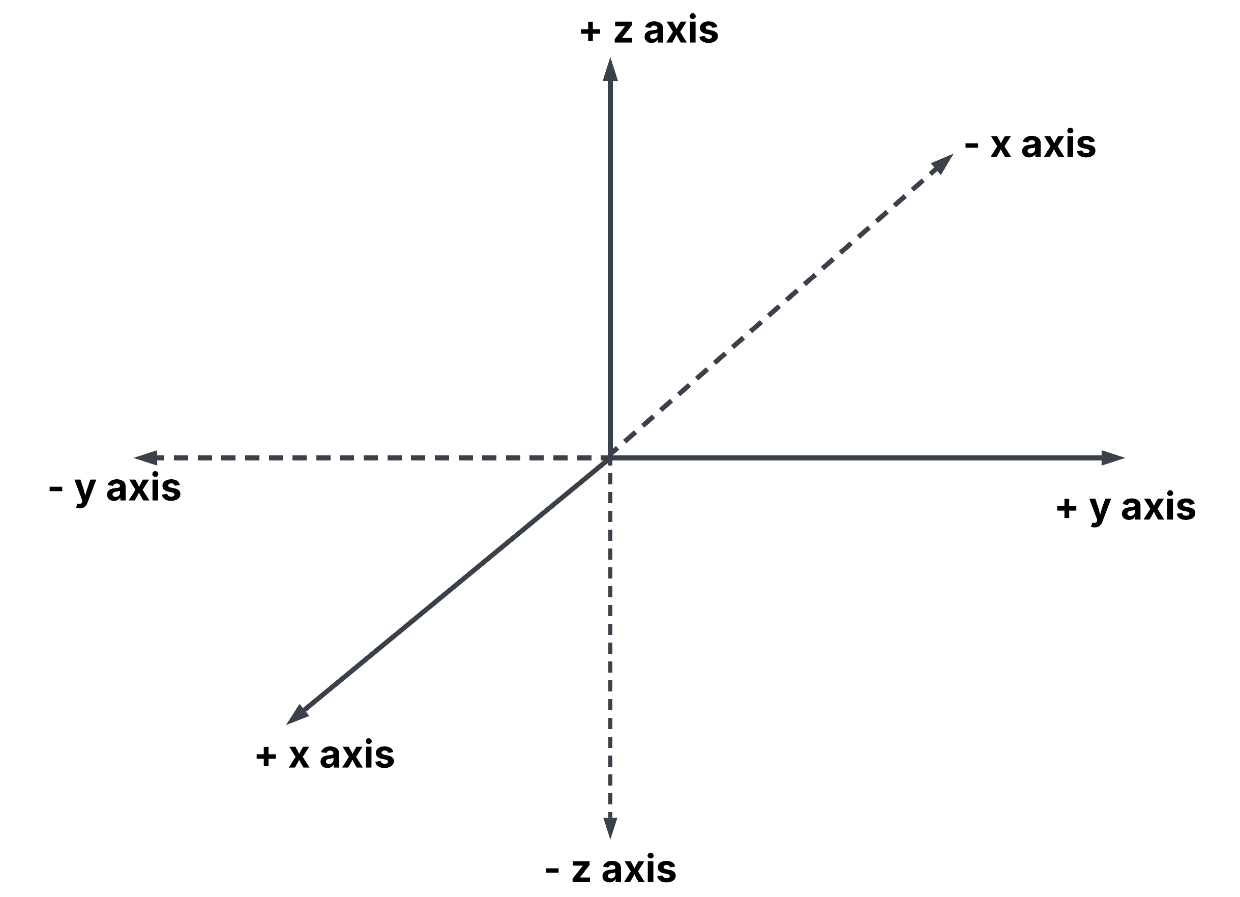
To describe fields mathematically, we often use the Cartesian Coordinate System (CCS), which represents a 2D or 3D space with coordinates ( $x$ and $y$ in 2D and $x$ , $y$ , and $z$ in 3D). Vector fields are defined using unit vectors $\boldsymbol{i}$ , $\boldsymbol{j}$ , $\boldsymbol{k}$ , corresponding to $x$ , $y$ , and $z$ directions:

3. The Del Operator in Vector Calculus

To analyze scalar and vector fields, we use a mathematical tool called the Del operator, denoted as $\nabla$ (nabla). It acts like a vector differential operator.

In a Cartesian system, the Del operator is defined as:

$\large\nabla = \begin{bmatrix}\frac{\partial}{\partial x} & \frac{\partial}{\partial y} & \frac{\partial}{\partial z}\end{bmatrix}$

This means that $\nabla$ operates on functions by taking their partial derivatives with respect to $x, y$ , and $z$ . Depending on how we apply it, we get different insights into scalar and vector fields:

Gradient $\mathbf{\nabla} F$ measures the rate and direction of change in a scalar field $F$
Divergence $\nabla \cdot \mathbf{F}$ tells us how much a vector field $F$ spreads out from or converges to a point.
Curl $\nabla \times \mathbf{F}$ captures the rotational tendency of a vector field $F$ .

4. The Concept of Gradient in a Scalar Field

Say you’re in a large building, looking for the strongest Wi-Fi signal. Since signal strength varies by location, it forms a scalar field, assigning a value (but not a direction) to every point.

Here’s the key question: how do we know which direction to walk in to get the strongest signal as quickly as possible? This is where the gradient comes in. It reveals two things: the direction in which the signal increases most rapidly, and how quickly that happens in that direction.

So, if at a spot with a weak signal, we should walk in the direction pointed to by the gradient of the signal.

4.1. Mathematical Formulation Using the Wi-Fi Analogy

Using the log-distance path loss model, we calculate how signal strength changes across space, and from there, compute the gradient to find the best direction for a stronger connection.

We begin with the formula for the signal strength $P(d)$ at distance $d$ from the router:

$P(d) = P_0 - 10n \log_{10} \left( \frac{d}{d_0} \right)$

Here, $P_0$ is the signal strength at reference distance $d_0$ , and $n$ is the path loss exponent (typically 2 to 4).

To understand how Wi-Fi signal strength varies across space, we calculate the gradient $\nabla P$ of the signal strength function $P$ :

$\nabla P =\begin{bmatrix}\frac{\partial P}{\partial x} & \frac{\partial P}{\partial y} & \frac{\partial P}{\partial z}\end{bmatrix}$

Since the signal strength $P$ depends on distance $d$ , and $d$ depends on spatial coordinates $x, y, z$ , we apply the chain rule.

First, we compute the derivative of $P(d)$ with respect to distance $d$ :

$\frac{\partial P}{\partial d} = -\frac{10n}{\ln(10)} \cdot \frac{1}{d}$

Since $P$ depends on $d$ , and $d=\sqrt{x^2 + y^2 +z^2}$ on $x, y, z$ , we’ll need partial derivatives of $d$ w.r.t. $x, y, z$ for the chain rule:

$\frac{\partial d}{\partial x} = \frac{x}{d}, \quad \frac{\partial d}{\partial y} = \frac{y}{d}, \quad \frac{\partial d}{\partial z} = \frac{z}{d}$

By combining these, we get:

$\nabla P = \left[-\frac{10n}{\ln(10)} \cdot \frac{x}{d^2}, -\frac{10n}{\ln(10)} \cdot \frac{y}{d^2}, -\frac{10n}{\ln(10)} \cdot \frac{z}{d^2} \right] = - \frac{10n}{\ln(10)}\frac{1}{d^2}[x, y, z]$

4.2. Worked Example

Suppose the router is at the origin $(0, 0, 0)$ , and we measure the signal at point $(3, 4, 5)$ . Given $P_o = -30$ dBm, $d_o = 1$ meter, and $n = 3$ , we first find the distance:

$d = \sqrt{3^2 + 4^2 + 5^2} \approx 7.07 \text{m}$

Next, using the signal strength model:

$P = -30 - 10 \cdot 3 \cdot \log_{10}(7.07) = -55.5 \, \text{dBm}.$

We compute the spatial gradient to examine how the signal strength changes with respect to position. First, we calculate the partial derivative of $P$ with respect to $x$ :

$\frac{\partial P}{\partial x} = -\frac{10n}{\ln(10)} \cdot \frac{x}{d^2} = -\frac{30}{\ln(10)} \cdot \frac{3}{50} \approx -0.7822$

Using the same method, we compute the $y$ and $z$ components of the gradient as well:

$\nabla P(3, 4, 5) \approx\begin{bmatrix}-0.7822 & -1.0424 & -1.3030\end{bmatrix}\ \text{dBm/m}$

Let’s interpret these results.

4.3. Interpretation

Negative values mean the signal strength weakens as we move away from the origin, whereas positive values mean the signal strengthens as we approach the origin.

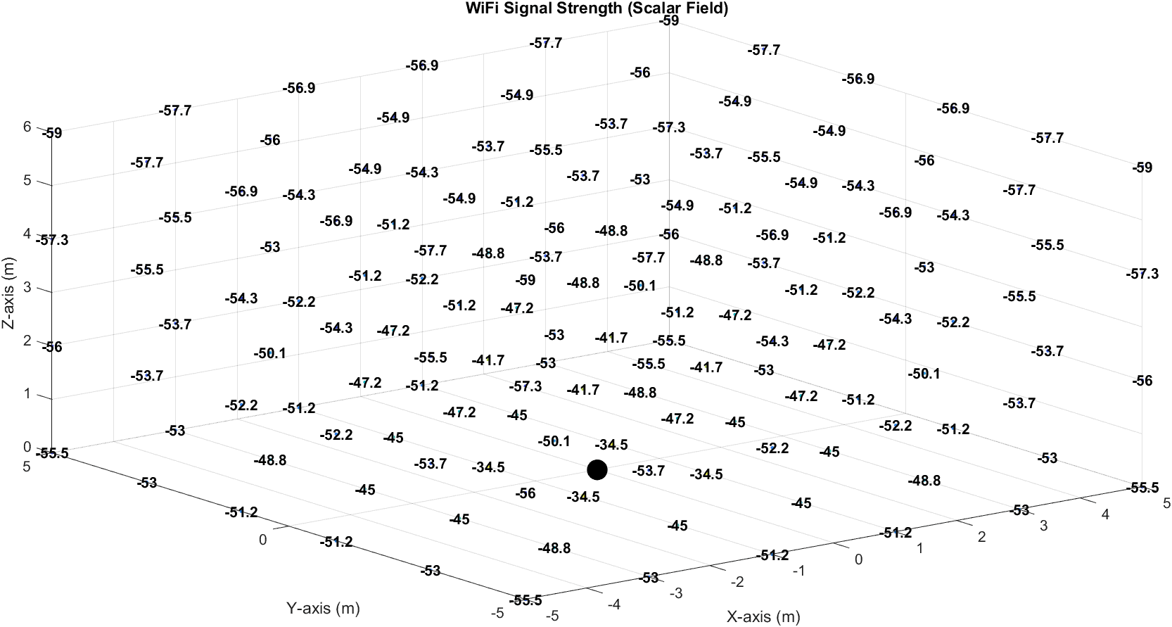
In our example, all the values are negative, and the most rapid drop occurs along the $z$ -axis, indicating that vertical shifts affect the signal strength the most. To improve the connection, we should move toward the origin of the router.

Here’s a 3D figure showing the scalar field of the signal strength:

Scalar field of the Wi-Fi signal strength

The corresponding gradient vectors are pointing towards the router:

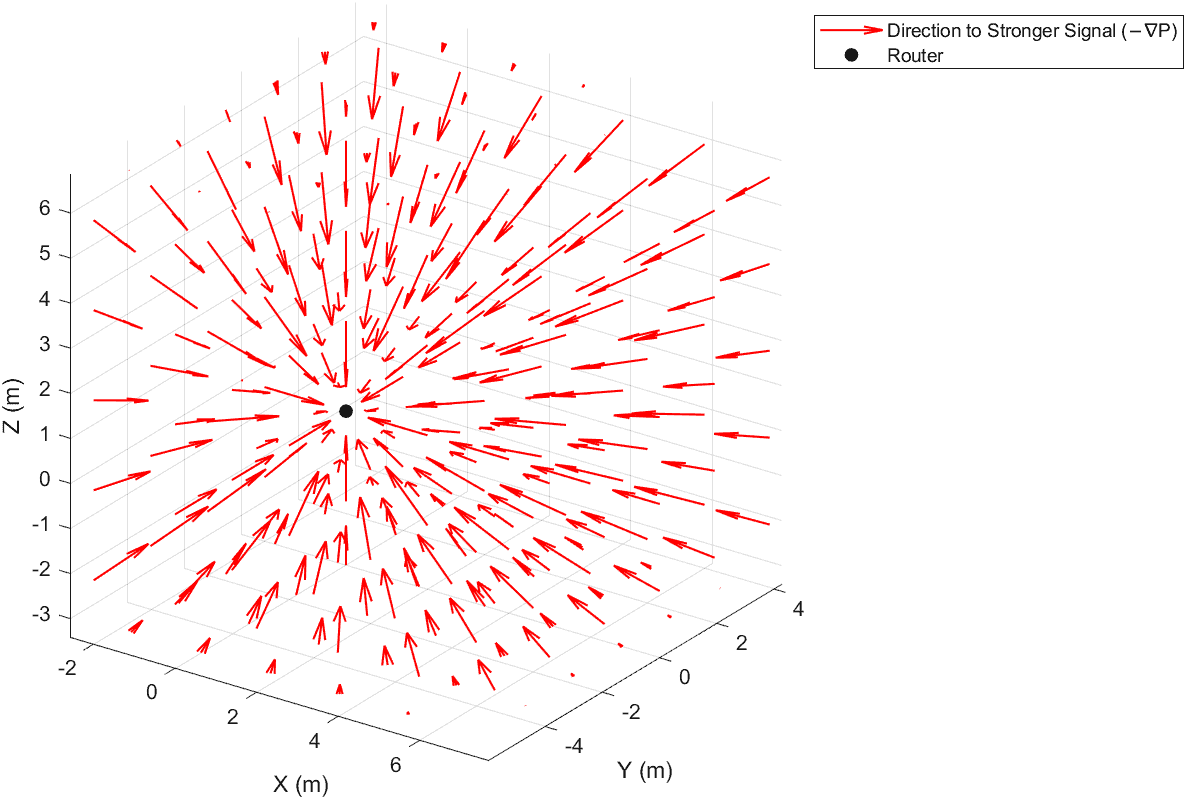
The gradient of a scalar field points in the direction of steepest increase, and moving in the opposite direction leads to the fastest decrease. This is the idea behind the gradient descent algorithm (GDA), a key method in machine learning used to minimize loss functions.

5. Divergence in a Vector Field

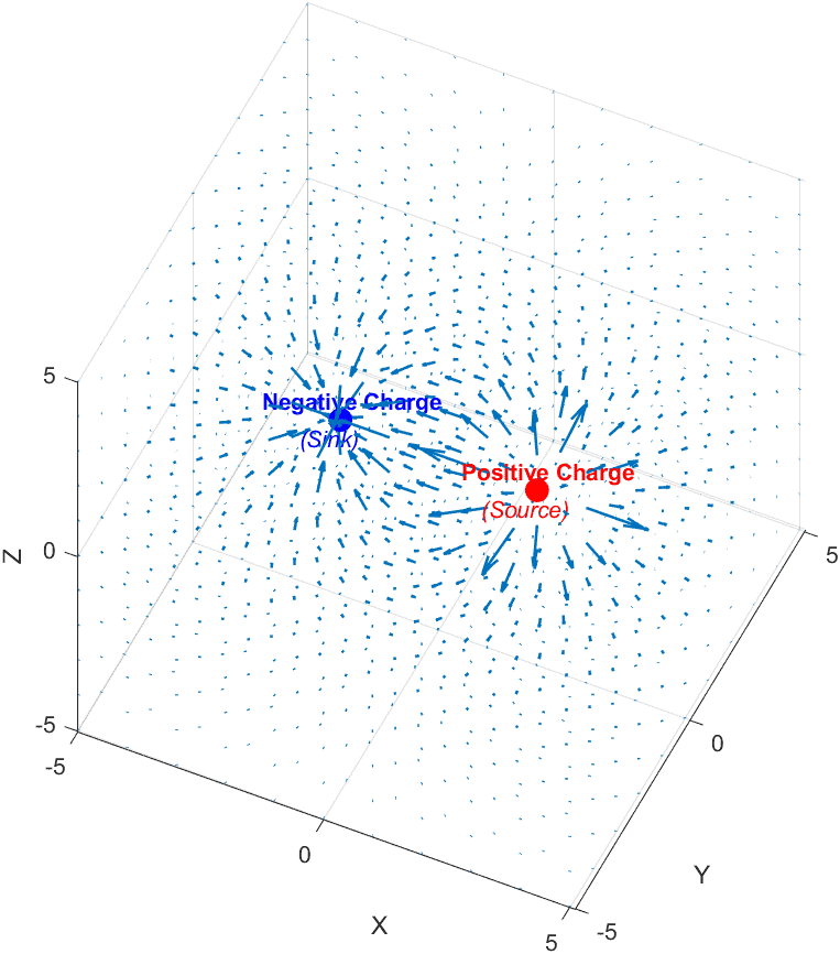
Let’s imagine this: drop a positive charge in space, and electric field lines instantly radiate outward like invisible arrows bursting from a source. With a negative charge, those arrows collapse inward toward it. That’s divergence at play.

Divergence reveals how much a vector field, such as an electric field, spreads from a point (a source) or converges into it (a sink).

The following figure illustrates this behavior:

Divergence of a Source and Sink in a vector field

Mathematically, for a vector field $\mathbf{F} = [F_x, F_y, F_z]$ , the divergence is given by:

$\mathbf{\nabla} \cdot \mathbf{F} = \frac{\partial F_x}{\partial x} + \frac{\partial F_y}{\partial y} + \frac{\partial F_z}{\partial z}$

This expression is the dot product of the del operator $\nabla$ and the vector field $\mathbf{F}$ in CCS.

When the divergence at a point is positive, the vector field behaves like a source at that specific location. If it’s negative, the point acts like a sink. And when the divergence is zero, the field is locally balanced there.

Let’s illustrate this concept.

5.1. A Smooth Polynomial Field Vector

Let’s consider a vector field $\mathbf{A} = [yz, 4xy, yz]$ . Let’s find the divergence $\nabla \cdot \mathbf{A}$ at the point .

We apply the divergence formula component-wise:

$\nabla \cdot \mathbf{A} = \frac{\partial A_x}{\partial x} + \frac{\partial A_y}{\partial y} + \frac{\partial A_z}{\partial z}$

Let’s compute each term:

$A_x = yz \Rightarrow \frac{\partial A_x}{\partial x} = 0 \quad \text{(no } x \text{ dependence)}$

$A_y = 4xy \Rightarrow \frac{\partial A_y}{\partial y} = 4x$

$A_z = yz \Rightarrow \frac{\partial A_z}{\partial z} = y$

Now plug in the point $(x, y, z) = (1, -2, 3)$ :

$\nabla \cdot \mathbf{A} = 0 + 4(1) + (-2) = 2$

So, the divergence at this point is 2, which means the field is acting like a source there.

6. The Curl of a Vector Field

Let’s say we’re beside a river and place a small paddlewheel in the water. If the water pushes evenly from all directions, the wheel stays still. However, if one side experiences a stronger flow, the wheel spins. That spin reflects the curl: it measures how much a vector field “swirls” around a point.

Mathematically, curl captures the field’s local rotation. For a vector field $\mathbf{F} = \begin{bmatrix} F_1 & F_2 & F_3 \end{bmatrix}$ , the curl is defined as:

$\mathbf{\nabla} \times \mathbf{F} = \begin{vmatrix} \mathbf{i} & \mathbf{j} & \mathbf{k} \\ \frac{\partial}{\partial x} & \frac{\partial}{\partial y} & \frac{\partial}{\partial z} \\ F_1 & F_2 & F_3 \end{vmatrix}$

Expanding this determinant, we get:

$\mathbf{\nabla} \times \mathbf{F} = \left( \frac{\partial F_3}{\partial y} - \frac{\partial F_2}{\partial z} \right)\mathbf{i} + \left( \frac{\partial F_1}{\partial z} - \frac{\partial F_3}{\partial x} \right)\mathbf{j} + \left( \frac{\partial F_2}{\partial x} - \frac{\partial F_1}{\partial y} \right)\mathbf{k}$

A zero curl means no rotation, i.e., the flow is smooth and straight. In contrast, a nonzero curl reveals spinning around the corresponding axis.

To determine the direction of that curl vector, we apply the right-hand rule. We point the fingers of our right hand in the direction of the flow that’s curving around, and the thumb will point in the direction of the curl:

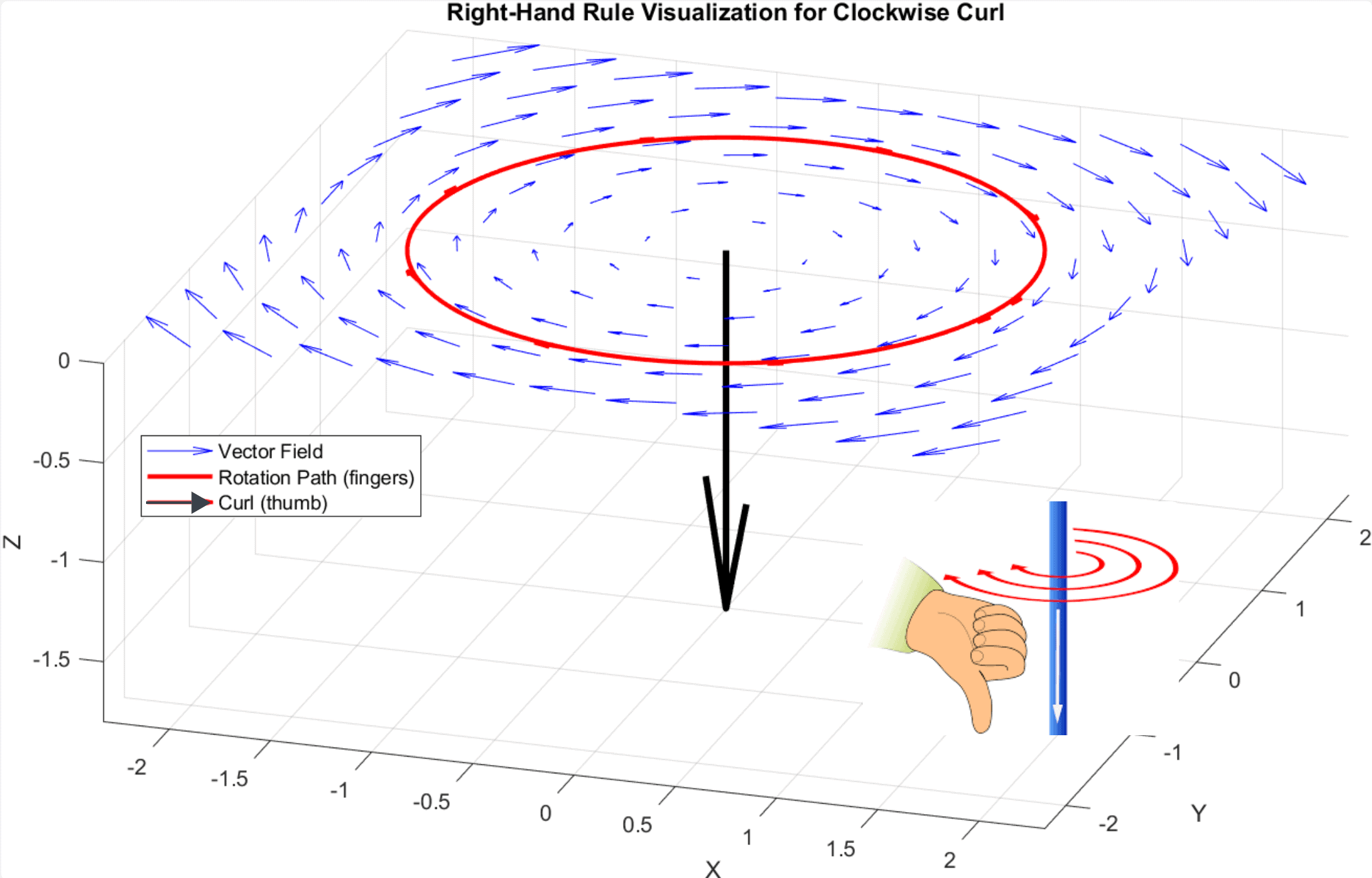
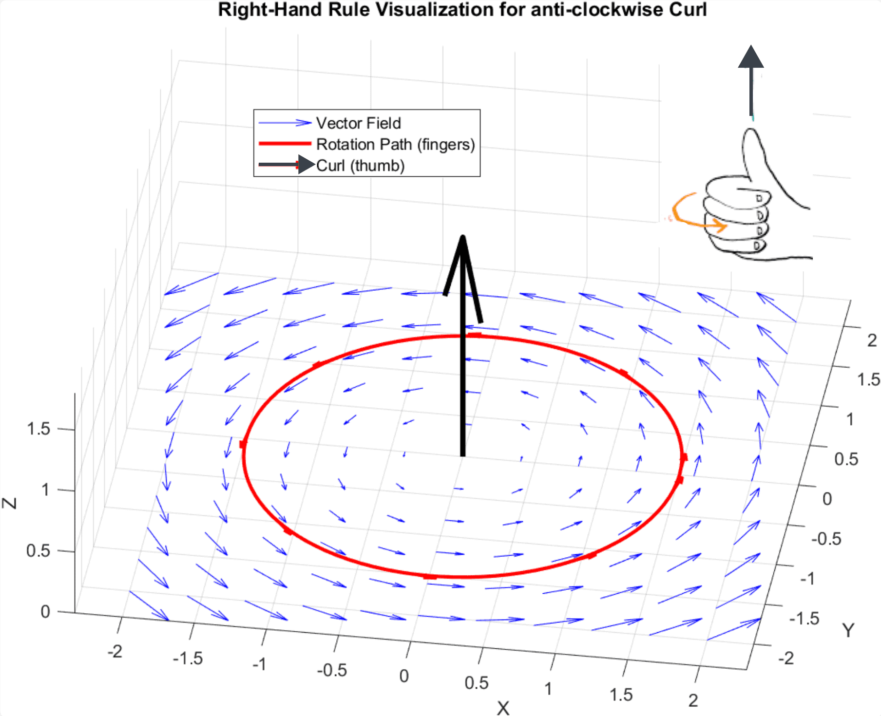
The curl’s magnitude tells us the rotation speed. The larger the magnitude, the faster the field swirls around that axis. If the curl is zero at a point, there’s no local spinning, just smooth, straight flow.

Let’s apply what we’ve just learned.

6.1. Case 1: A Field with No Curl

Consider the vector field:

$\mathbf{F} =\begin{bmatrix}yz & xz & xy\end{bmatrix}$

To compute the curl, we evaluate:

$\frac{\partial F_3}{\partial y} - \frac{\partial F_2}{\partial z} = x - x = 0$

$\frac{\partial F_1}{\partial z} - \frac{\partial F_3}{\partial x} = y - y = 0$

$\frac{\partial F_2}{\partial x} - \frac{\partial F_1}{\partial y} = z - z = 0$

As a result, every component of the curl vanishes:

$\mathbf{\nabla} \times \mathbf{F} = \mathbf{0}$

This means the field has no rotational effect. While the flow exists, it’s entirely non-rotational. So, placing a paddlewheel anywhere in this field leaves it motionless:

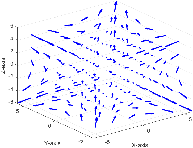
An irrotational or curl-free vector field

In this field, the arrows neither swirl nor form loops around any axis. Using the right-hand rule, we cannot establish a definite circular path. This tells us the field is irrotational, meaning its curl is zero.

6.2. Case 2: A Rotating Field

Now, let’s tweak the field to introduce rotation:

$\mathbf{F} =\begin{bmatrix}-y & x & 0\end{bmatrix}$

Computing the curl yields:

$\frac{\partial F_3}{\partial y} - \frac{\partial F_2}{\partial z} = 0 - 0 = 0$

$\frac{\partial F_1}{\partial z} - \frac{\partial F_3}{\partial x} = 0 - 0 = 0$

$\frac{\partial F_2}{\partial x} - \frac{\partial F_1}{\partial y} = 1 - (-1) = 2$

So, we get:

$\mathbf{\nabla} \times \mathbf{F} = 2\mathbf{k}$

Clearly, the field rotates about the $z$ -axis, much like a whirlpool swirling on a lake’s surface.

The next figure shows this in action:

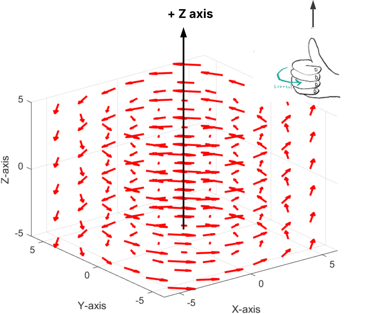
When we apply the right-hand rule, our thumb points upward along the Z-axis.

7. Conclusion

In this article, we explored the meaning behind three core vector calculus tools: the gradient, curl, and divergence.

The gradient points in the direction of the steepest increase of a scalar field, the divergence tells us how much a vector field spreads out from or converges to a point, and the curl measures the local rotation of a field.

The post What Are Gradient, Divergence, and Curl in Vector Calculus? first appeared on Baeldung on Computer Science.